
本文是A Tutorial on Thompson Sampling的学习笔记。在阅读该文前,可能需要对贝叶斯统计有一定的了解。
Background
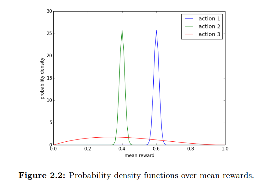
在强化学习中,有一个explore和exploit的平衡(可以看这个Explore-exploit tradeoff)。通常我们会使用-greedy的策略,但是这个策略也有缺点,就是对于非最优的action采取了同样的选择概率。
What’s Thompson Sampling
和Greedy Decision对比可以很好的说明什么是Thompson sampling,两者算法流程图如下:
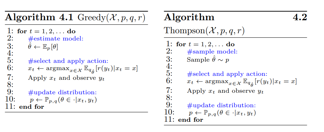
可以看到,左边的贪婪算法,相当于从后验分布中选取了期望值作为模型参数,而Thompson Sampling则是从 的后验分布中进行采样。
code Framework
Thompson Sampling的远离还是很简单的,在介绍完下面的RL实验框架后,就开始看code。
在RL中我们会有三个抽象对象,一个是environment,一个是agent,另一个是scheduler用来调度environment和agent交互。
scheduler
scheduler主要实现以下run_one_step,在每一步交互中完成以下动作:
environment得到观测;agent通过观测选择对应的action;environment通过所做出的动作给出agent某种回报;agent通过得到的回报用以改善动作决策模型。
class BaseScheduler(object):
    def __init__(self, agent, environment, n_steps,
                seed=0, rec_freq=1, unique_id='NULL'):
        self.agent = agent
        self.environment = environment
        self.n_steps = n_steps

    def run_one_step(self, t):
        observation = self.environment.get_observation()
        action = self.agent.pick_action(observation)

        optimal_reward = self.environment.get_optimal_reward()
        expected_reward = self.environment.get_expected_reward(action)
        reward = self.environment.get_stochastic_reward(action)


        self.agent.update_observation(observation, action, reward)

        instant_regret = optimal_reward - expected_reward
        self.cum_regret += instant_regret

        self.environment.advance(action, reward)

    def run_experiment(self):
        np.random.seed(self.seed)
        self.cum_regret = 0
        self.cum_optimal = 0

        for t in range(self.n_steps):
            self.run_one_step(t)
environment
environment主要实现了上述的
get_observation;get_optimal_reward,该方法是当前最佳动作所产生的回报,跟agent无关;get_expected_reward,该方法时environment根据动作产出回报的期望,仅用以度量表现使用;get_stochastic_reward,该方法是实际agent得到的回报;advance,更新环境。
agent
agent主要实现了上述的
pick_action,根据传入的观测选择动作;update_observation,根据(observation, action, reward)三维数组更新决策模型。
Conjugate prior
接下来,我们通过一些例子和代码来看上述方法都是怎么实现的。
Multi-armed bandit
既然Thompson Sampling要推断后验分布,最简单的形式还是共轭分布(这里姑且这么叫吧)。
这个例子是一个多臂老虎机,先验分布是一个beta分布,似然是一个binomial分布,出来的后验还是一个beta分布。
由于environment观测比较简单,就是一个有几个遥感,这里就直接看agent的接口:
def pick_action(self, observation):
    if np.random.rand() < self.epsilon:
        action = np.random.randint(self.n_arm)
    else:
        posterior_means = self.get_posterior_mean()
        action = random_argmax(posterior_means)

    return action

def get_posterior_mean(self):
    return self.prior_success / (self.prior_success + self.prior_failure)

def update_observation(self, observation, action, reward):
    assert observation == self.n_arm

    if np.isclose(reward, 1):
      self.prior_success[action] += 1
    elif np.isclose(reward, 0):
      self.prior_failure[action] += 1
    else:
      raise ValueError('Rewards should be 0 or 1 in Bernoulli Bandit')
binomial bridge
Binomial bridge的形状是这个样子:
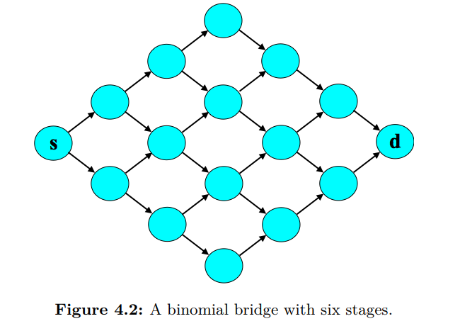
这里的场景是,每个边的用时都遵循一个期望是 ,方差是 的 log-normal 分布(分布性质可参阅 log-normal wiki,对数正态分布)。同时我们让 的也遵循期望是 ,方差是 的 log-normal 分布。其后验更新方式如下:
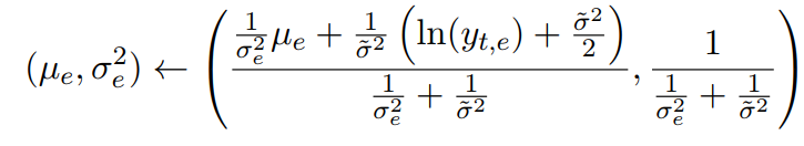
TODO:解释为什么这么更新。
How to approximate the posterior
虽然共轭先验的形式,我们可以有一个解析的更新方式,但是对于更一般的情况下,我们该如何求解呢?
Gibbs Sampling
Laplace Approximation
Laplace approximation 通过对概率密度函数 在其极值点,,进行二阶泰勒展开,以 为均值,为方差的高斯分布来近似原分布。
当以下环境下,其方法比较适用:
- 后验的极值,hessian矩阵很好计算时;
- 分布在聚集在极值点附近。
Bootstrap
Bootstrap是通过对历史的样本进行均匀的有放回采样得到新的模拟样本,在这个样本上计算出极值用来当成当前模型参数。
在文中,作者提及Bootstrap方法是没有理论保证一定work的。
Summary
这里我们略去计算部分(在之后的application中会涉及计算),只关注于他们的框架,
Bootstrap
def _resample_history(self, random=True):
    """Generates a resampled version of the history.
    If random = False, then no resampling is done."""

    if self.history_size > 0:
      if random:
        random_indices = np.random.randint(0, self.history_size,
                                           self.history_size)
        resampled_feedback_history = []
        resampled_path_hitory = []
        for ind in random_indices:
          resampled_feedback_history.append(self.feedback_history[ind])
          resampled_path_hitory.append(self.path_history[ind])

        self.resampled_path_history = resampled_path_hitory
        self.resampled_feedback_history = resampled_feedback_history
      else:
        self.resampled_path_history = self.path_history
        self.resampled_feedback_history = self.feedback_history

def get_sample(self):
    # resampling the history
    self._resample_history()

    # flattened sample
    flattened_sample, _ = self._optimize_Newton_method()

    # making sure all the samples are positive
    flattened_sample = np.maximum(flattened_sample, _SMALL_NUMBER)

    edge_length = copy.deepcopy(self.internal_env.graph)

    for start_node in edge_length:
      for end_node in edge_length[start_node]:
        edge_index = self.edge2index[start_node][end_node]
        edge_length[start_node][end_node] = flattened_sample[edge_index]

    return edge_length

def pick_action(self, observation):
    """Greedy shortest path wrt bootstrap sample."""
    bootstrap_sample = self.get_sample()
    self.internal_env.overwrite_edge_length(bootstrap_sample)
    path = self.internal_env.get_shortest_path()

    return path
Laplace Approximation
  def get_sample(self):
    """Sets the bootstrap sample for each edge length

    Return:
      edge_length - dict of dicts edge_length[start_node][end_node] = distance
    """
    # resampling the history
    self._resample_history(False)

    # flattened sample
    x_map, hessian = self._optimize_Newton_method(True)
    cov = npla.inv(-hessian)
    flattened_sample = np.random.multivariate_normal(x_map, cov)

    # making sure all the samples are positive
    flattened_sample = np.maximum(flattened_sample, _SMALL_NUMBER)

    edge_length = copy.deepcopy(self.internal_env.graph)

    for start_node in edge_length:
      for end_node in edge_length[start_node]:
        edge_index = self.edge2index[start_node][end_node]
        edge_length[start_node][end_node] = flattened_sample[edge_index]

    return edge_length
Application
Article Recommendation
在时刻 ,我们观察到具有特征 的顾客,向其推荐具有特征 的文章 ,顾客阅读的可能性为 , 是我们需要学习的参数, 服从高斯分布先验。
下面两个函数分别用以计算高斯分布先验梯度和hessian,逻辑回归梯度和hessian。
def _compute_gradient_hessian_prior(self,x):
    Sinv = np.diag([1/self.theta_std**2]*self.dim)
    mu = self.theta_mean*np.ones(self.dim)

    g = Sinv.dot(x - mu)
    H = Sinv

    return g,H

def _compute_gradient_hessian(self,x,article):

    g,H = self._compute_gradient_hessian_prior(x)

    for i in range(self.num_plays[article]):
      z = self.contexts[article][i]
      y = self.rewards[article][i]
      pred = 1/(1+np.exp(-x.dot(z)))

      g = g + (pred-y)*z
      H = H + pred*(1-pred)*np.outer(z,z)
Product Assortment
loading…